Yapay Sinir Ağı Ağırlıklarının Görselleştirilmesi

Yapay sinir ağları, özünde her katmanda yapılan matris çarpımlarından oluşur. Bu çarpımlar doğrusal dönüşümlerdir. Bu görselleştirme, katmanlardaki doğrusal dönüşümleri ve her katmanın kayıp yüzeyini gösterir. Bu not defteri, Yapay Sinir Ağı not defterinin devamı niteliğindedir. Geri yayılımın türetilmesi ve yapay sinir ağlarının matematiksel arka planı için bir önceki not defterine bakabilirsiniz.

Gavin’in notu: Bu görselleştirmenin amacı, geri yayılımın ağırlıkları ve bias değerlerini en uygun biçimde güncellediğini göstermektir. Bunu görünür kılmak için program, ağırlıkları bilerek optimumdan uzaklaştırıyor ve kaybın nasıl arttığını gösteriyor. Bu nedenle çalışması oldukça uzun sürer.

import numpy as np
import torch
import torch.nn as nn
import torch.nn.functional as F

# %matplotlib ipympl
import matplotlib.pyplot as plt
from mpl_toolkits.mplot3d import Axes3D

from celluloid import Camera
import scienceplots
from IPython.display import Image

torch.manual_seed(0)
np.random.seed(0)
plt.style.use(["science", "no-latex"])

Eğitim Veri Kümesi

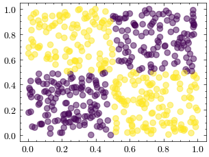
Doğrusal olmayan bir veri kümesi oluşturalım. Yapay sinir ağları bu fonksiyona uyabilirken, perceptron gibi doğrusal modeller bu veri kümesinde yakınsayamaz.

# generate the non-linear dataset, meaning that a hiper düzlem can't separate the data
def generate_XOR():
    N = 500
    X = np.random.rand(N, 2)
    y = (X[:, 0] > 0.5) != (X[:, 1] > 0.5)

    return X, y


X, y = generate_XOR()

fig = plt.figure()
ax = fig.add_subplot()
ax.scatter(X[:, 0], X[:, 1], c=y, alpha=0.5)

<matplotlib.collections.PathCollection at 0xffff2f2330e0>

Grafik Fonksiyonları

Eğitim fonksiyonunda optimizer, ağırlıkları güncelleyip bir sonraki adıma geçmemizi sağlar. Peki ya optimizer’ın önerdiği ağırlıkları kullanmasaydık? Buradaki grafik fonksiyonları, sinir ağındaki katmanların ağırlık matrisindeki değerleri elle değiştirip ağı yeniden çalıştırarak kaybın nasıl değiştiğini gösterir.

Ayrıca her katmandaki doğrusal dönüşümü ayrı ayrı gösteren grafik fonksiyonları da bulunur.

def create_scatterplots(rows=2, cols=3, width_scale=1, height_scale=1):
    fig, axes = plt.subplots(
        rows,
        cols,
        figsize=(16 / 9.0 * 4 * width_scale, 4 * height_scale),
        layout="constrained",
    )
    axes = axes.flatten()

    layer_idx = 0
    for i, axis in enumerate(axes):
        if not ((i + 1) % cols == 0):
            axis.set_title(f"Katman {layer_idx}")
            layer_idx += 1

    axes[-1].set_title("Tahminler")
    axes[-1 - cols].set_title("Ortalama Karesel Hata")

    camera = Camera(fig)
    return axes, camera


def create_3d_plots(rows=2, cols=3, width_scale=1, height_scale=1):
    fig = plt.figure(
        figsize=(16 / 9.0 * 4 * width_scale, 4 * height_scale), layout="constrained"
    )
    axes = []

    layer_idx = 0
    for i in range(rows * cols):
        if not ((i + 1) % cols == 0):
            axis = fig.add_subplot(rows, cols, i + 1, projection="3d")
            axis.set_title(f"Katman {layer_idx + 1}")
            axes.append(axis)
            layer_idx += 1
        else:
            axes.append(fig.add_subplot(rows, cols, i + 1))

    axes[-1].set_title("Tahminler")
    axes[-1 - cols].set_title("Ortalama Karesel Hata")

    camera = Camera(fig)
    return axes, camera


def plot_layer_loss_landscape(
    axis,
    model,
    target_layer_idx,
    neuron_idx,
    features,
    labels,
    w1_min,
    w1_max,
    w2_min,
    w2_max,
    loss_dims,
    device,
    color="blue",
):
    """İlk nörondaki ilk iki ağırlık değiştiğinde kaybın nasıl değiştiğini çiz"""
    loss_fn = nn.MSELoss()

    init = model.get_values(target_layer_idx, neuron_idx)
    w1 = init[0].item()
    w2 = init[1].item()

    target_layer_idx = target_layer_idx % len(model.layers)

    w1_range = torch.linspace(w1_min + w1, w1_max + w1, loss_dims).to(device)
    w2_range = torch.linspace(w2_min + w2, w2_max + w2, loss_dims).to(device)
    w1_range, w2_range = torch.meshgrid(w1_range, w2_range, indexing="ij")
    w_range = torch.stack((w1_range.flatten(), w2_range.flatten()), axis=1)

    error_range = np.array([])

    for target_layer_weight in w_range:
        model.override_layer_weight(
            target_layer_idx, neuron_idx, init + target_layer_weight
        )
        error = 0
        for x, y in zip(features, labels):
            output = model(x)
            y = y.unsqueeze(0)
            loss = loss_fn(output, y)
            error += loss.detach().cpu().numpy()
        error /= len(labels)
        error_range = np.append(error_range, error)

        if np.isclose(target_layer_weight[0].item(), w1, atol=0.25) and np.isclose(
            target_layer_weight[1].item(), w2, atol=0.25
        ):
            axis.scatter([w1], [w2], [error], color=color, alpha=0.4)

    axis.plot_surface(
        w1_range.detach().cpu().numpy(),
        w2_range.detach().cpu().numpy(),
        error_range.reshape(loss_dims, loss_dims),
        color=color,
        alpha=0.1,
    )
    model.override_layer_weight(target_layer_idx, neuron_idx, init)


def plot_mse_and_predictions(
    axes, features, idx, visible_mse, mse_idx, errors, predictions, cmap, cols, device
):
    features_cpu = features.detach().cpu().numpy()

    # Plot MSE
    mse_ax = axes[-1 - cols]
    mse_ax.plot(
        mse_idx[visible_mse][: idx + 1],
        errors[visible_mse][: idx + 1],
        color="red",
        alpha=0.5,
    )
    mse_ax.plot(
        [1],
        [0],
        color="white",
        alpha=0,
    )

    # Plot Tahminler
    predictions_classes = np.where(predictions > 0.5, 1, 0)

    predictions_ax = axes[-1]
    predictions_ax.scatter(
        features_cpu[:, 0],
        features_cpu[:, 1],
        c=predictions_classes,
        cmap=cmap,
        alpha=0.5,
    )


def plot_transformations_and_predictions(
    axes,
    model,
    idx,
    visible_mse,
    mse_idx,
    errors,
    predictions,
    features,
    labels,
    cmap,
    rows,
    cols,
    device,
):
    plot_mse_and_predictions(
        axes,
        features,
        idx,
        visible_mse,
        mse_idx,
        errors,
        predictions,
        cmap,
        cols,
        device,
    )
    model.visualize(features, labels, axes, cmap, rows, cols)


def plot_loss_landscape_and_predictions(
    axes,
    model,
    idx,
    visible_mse,
    mse_idx,
    errors,
    predictions,
    features,
    labels,
    cmap,
    cols,
    device,
    w1_min=-5,
    w1_max=5,
    w2_min=-5,
    w2_max=5,
    loss_dims=7,
):
    # this uses axes with index -1 and -1-cols
    plot_mse_and_predictions(
        axes,
        features,
        idx,
        visible_mse,
        mse_idx,
        errors,
        predictions,
        cmap,
        cols,
        device,
    )

    num_layers = len(model.layers)

    target_layer_idx = -1

    for index, axis in enumerate(reversed(axes)):
        # in reverse order, predictions plot is index 0 and mse plot is index cols
        if index == 0 or index == cols or abs(target_layer_idx) > num_layers:
            continue
        plot_layer_loss_landscape(
            axis,
            model,
            target_layer_idx,
            0,
            features,
            labels,
            w1_min,
            w1_max,
            w2_min,
            w2_max,
            loss_dims,
            device,
            color="blue",
        )
        if target_layer_idx != -1:
            plot_layer_loss_landscape(
                axis,
                model,
                target_layer_idx,
                1,
                features,
                labels,
                w1_min,
                w1_max,
                w2_min,
                w2_max,
                loss_dims,
                device,
                color="red",
            )
        target_layer_idx -= 1

PyTorch ile Uygulama

PyTorch kullanarak ileri beslemeli bir yapay sinir ağı tanımlayalım; ancak bu kez her katmana ağırlıkları elle değiştirebilen özel fonksiyonlar da ekleyelim. Amacımız, ağırlıklar optimum noktada olmadığında kaybın nasıl davrandığını görmek. Böylece geri yayılımın ağırlıkları neden en iyi şekilde güncellediğini görselleştirebiliriz.

class VisualNet(nn.Module):
    def __init__(self):
        super(VisualNet, self).__init__()
        self.layers = nn.ModuleList()

    def visualize(self, X, y, axes, cmap, rows, cols):
        y_cpu = y.detach().cpu().numpy()

        layer_idx = 0
        for i, axis in enumerate(axes):
            if not ((i + 1) % cols == 0):
                X_cpu = X.detach().cpu().numpy()

                # input and hidden layer outputs
                if X.shape[1] != 1:
                    axis.scatter(
                        X_cpu[:, 0], X_cpu[:, 1], c=y_cpu, cmap=cmap, alpha=0.5
                    )
                # output layer is 1D, so set second dimenstional to zeros
                else:
                    axis.scatter(
                        X_cpu[:, 0],
                        np.zeros(X_cpu[:, 0].shape),
                        c=y_cpu,
                        cmap=cmap,
                        alpha=0.5,
                    )

                if layer_idx < len(self.layers):
                    X = F.tanh(self.layers[layer_idx](X))
                    layer_idx += 1

    def override_layer_weight(self, layer_idx, neuron_idx, new_weights):
        if (abs(layer_idx) > len(self.layers)) or (
            abs(neuron_idx) > len(self.layers[layer_idx].weight)
        ):
            return

        with torch.no_grad():
            self.layers[layer_idx].weight[neuron_idx, :2] = new_weights

    def get_values(self, layer_idx, neuron_idx):
        if (abs(layer_idx) > len(self.layers)) or (
            abs(neuron_idx) > len(self.layers[layer_idx].weight)
        ):
            return torch.zeros(2)

        with torch.no_grad():
            return self.layers[layer_idx].weight.detach().clone()[neuron_idx, :2]


class TorchNet(VisualNet):
    def __init__(self, num_hidden_layers):
        super().__init__()

        # define the layers
        self.input_layer = nn.Linear(2, 2)
        self.layers.append(self.input_layer)

        for i in range(num_hidden_layers):
            self.layers.append(nn.Linear(2, 2))

        self.output_layer = nn.Linear(2, 1)
        self.layers.append(self.output_layer)

    def forward(self, x):
        # pass the result of the previous layer to the next layer
        for layer in self.layers[:-1]:
            x = F.tanh(layer(x))

        return self.output_layer(x)

Modeli Eğitmek

Bir önceki Yapay Sinir Ağı not defterinde olduğu gibi, eğitim verisini modele verecek, optimizer ile ağırlıkları güncelleyecek ve görselleştirmeyi yenileyeceğiz.

def torch_fit(
    model,
    features,
    labels,
    epochs,
    learning_rate,
    transformations_plot_filename,
    loss_landscape_plot_filename,
    device,
    rows=2,
    cols=3,
    width_scale=1,
    height_scale=1,
):
    mse_idx = np.arange(1, epochs + 1)
    errors = np.full(epochs, -1)

    cmap = plt.cm.colors.ListedColormap(["red", "blue"])

    scatterplots, camera1 = create_scatterplots(rows, cols, width_scale, height_scale)
    loss_plots, camera2 = create_3d_plots(rows, cols, width_scale, height_scale)

    loss_fn = nn.MSELoss()
    optimizer = torch.optim.SGD(model.parameters(), lr=learning_rate, momentum=0.3)

    for idx in range(epochs):
        error = 0
        predictions = np.array([])

        for x, y in zip(features, labels):
            # Forward Propagation
            output = model(x)

            output_np = output.detach().cpu().numpy()
            predictions = np.append(predictions, output_np)

            # Store Hata
            # tensor(0.) -> tensor([0.]) to match shape of output variable
            y = y.unsqueeze(0)
            loss = loss_fn(output, y)

            error += loss.detach().cpu().numpy()

            # Backpropagation
            optimizer.zero_grad()
            loss.backward()
            optimizer.step()

        if (
            idx < 5
            or (idx <= 50 and idx % 5 == 0)
            or (idx <= 1000 and idx % 50 == 0)
            or idx % 250 == 0
        ):
            print(f"epok: {idx}, MSE: {error}")

            # Plot MSE
            errors[idx] = error
            visible_mse = errors != -1

            plot_transformations_and_predictions(
                scatterplots,
                model,
                idx,
                visible_mse,
                mse_idx,
                errors,
                predictions,
                features,
                labels,
                cmap,
                rows,
                cols,
                device,
            )

            plot_loss_landscape_and_predictions(
                loss_plots,
                model,
                idx,
                visible_mse,
                mse_idx,
                errors,
                predictions,
                features,
                labels,
                cmap,
                cols,
                device,
            )

            camera1.snap()
            camera2.snap()

    animation1 = camera1.animate()
    animation1.save(transformations_plot_filename, writer="pillow")
    animation2 = camera2.animate()
    animation2.save(loss_landscape_plot_filename, writer="pillow")

    plt.show()

Dönüşümleri ve Ağırlık Güncellemelerini Görselleştirmek

Görselleştirmeyi üretmek için eğitim fonksiyonunu modelimizle birlikte çağıralım.

device = torch.device("cuda:0" if torch.cuda.is_available() else "cpu")
torch_model = TorchNet(num_hidden_layers=2).to(device)

rows = 2
cols = 3

# the inputs and outputs for PyTorch must be tensors
X_tensor = torch.tensor(X, device=device, dtype=torch.float32).squeeze(-1)
y_tensor = torch.tensor(y, device=device, dtype=torch.float32).squeeze(-1)

epochs = 601
learning_rate = 0.005

transformations_plot_filename = "neural_network_weights.gif"
loss_landscape_plot_filename = "neural_network_weights_loss_landscape.gif"
torch_fit(
    torch_model,
    X_tensor,
    y_tensor,
    epochs,
    learning_rate,
    transformations_plot_filename,
    loss_landscape_plot_filename,
    device,
    rows=rows,
    cols=cols,
)

epok: 0, MSE: 137.9026336669922
epok: 1, MSE: 127.58297729492188
epok: 2, MSE: 127.3271713256836
epok: 3, MSE: 127.13655853271484
epok: 4, MSE: 126.98948669433594
epok: 5, MSE: 126.87287139892578
epok: 10, MSE: 126.53106689453125
epok: 15, MSE: 126.36543273925781
epok: 20, MSE: 126.266357421875
epok: 25, MSE: 126.19721984863281
epok: 30, MSE: 126.14079284667969
epok: 35, MSE: 126.08564758300781
epok: 40, MSE: 126.01984405517578
epok: 45, MSE: 125.92532348632812
epok: 50, MSE: 125.76524353027344
epok: 100, MSE: 95.95246124267578
epok: 150, MSE: 56.10152053833008
epok: 200, MSE: 54.98665237426758
epok: 250, MSE: 38.98552703857422
epok: 300, MSE: 20.435640335083008
epok: 350, MSE: 13.933258056640625
epok: 400, MSE: 11.308575630187988
epok: 450, MSE: 9.152091979980469
epok: 500, MSE: 7.561526298522949
epok: 550, MSE: 6.4366888999938965
epok: 600, MSE: 5.587584018707275

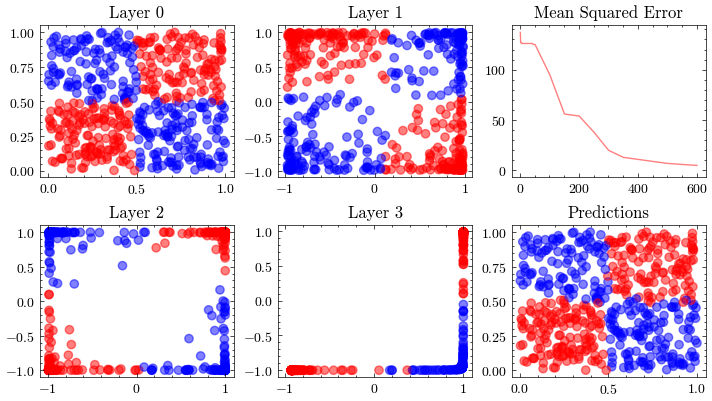
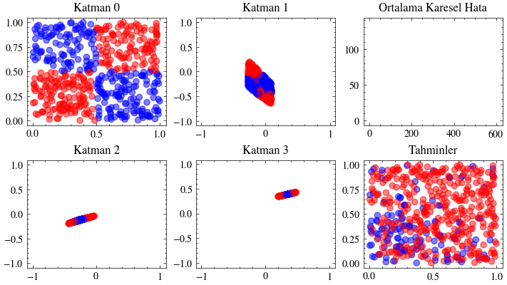
Bu görselleştirme, sinir ağındaki her katmanın iç doğrusal dönüşümünü gösterir. Her katmanın girdiyi nasıl bir çıktıya dönüştürdüğünü adım adım izleyeceğiz. Üçüncü katmanda verinin doğrusal olarak ayrılabilir hale geldiğini göreceksiniz. İşte bu dönüşümler sayesinde ağ, girdileri iki sınıfa ayırmayı başarır.

Image(filename=transformations_plot_filename)

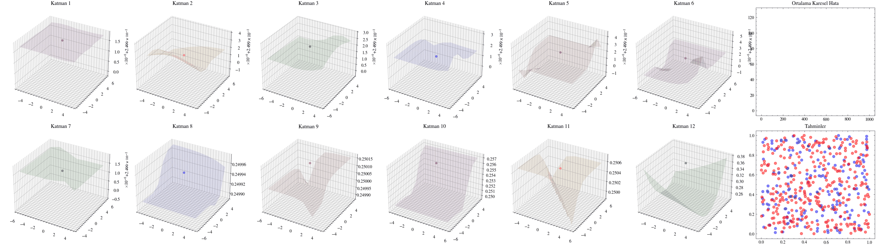
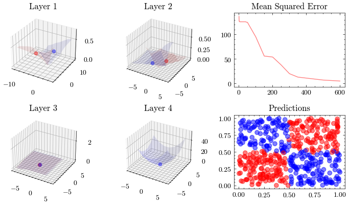
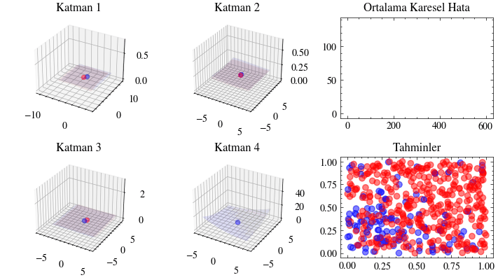
Bu görselleştirme, son katmandaki kayıp fonksiyonu minimuma yaklaşırken tüm ağırlıkların birlikte nasıl güncellendiğini gösterir. Dördüncü katmandaki 3B grafiğin minimum noktaya yerleştiğine dikkat edin.

Image(filename=loss_landscape_plot_filename)

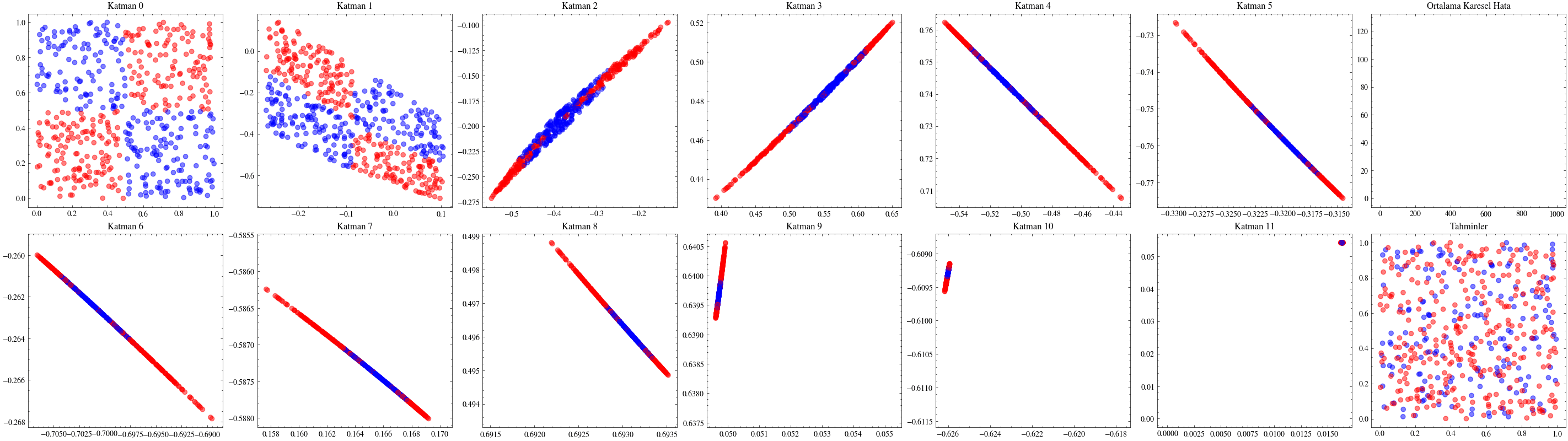
Kaybolan Gradyanlar

Katman sayısını artırmanın ağın daha fazla örüntü öğrenmesini sağlayacağı düşüncesi ilk bakışta mantıklıdır. Ancak ölçekleme her zaman bu kadar doğrudan işlemez. Yanlış mimariler seçildiğinde ağlar derinleştikçe öğrenmeyi sürdüremez. Bir sonraki görselleştirmede katman sayısını 12’ye çıkaracağız ve ağırlıkların artık güncellenemediğini göreceğiz. Buna kaybolan gradyan sorunu denir: ağa geriye doğru taşınan güncellemeler, ilk katmanlara ulaştığında sıfıra çok yaklaştığı için ağırlıklar neredeyse hiç değişmez. ResNet makalesindeki residual bağlantılar, bu sorunun hafifletilmesinde önemli bir adım olmuştur.

12 Katmanlı Yapay Sinir Ağı

Bu kez aynı kodu daha büyük bir ağ ile yeniden çalıştıralım.

device = torch.device("cuda:0" if torch.cuda.is_available() else "cpu")
torch_model = TorchNet(num_hidden_layers=10).to(device)

rows = 2
cols = 7

X_tensor = torch.tensor(X, device=device, dtype=torch.float32).squeeze(-1)
y_tensor = torch.tensor(y, device=device, dtype=torch.float32).squeeze(-1)

epochs = 1001
learning_rate = 0.005

width_scale = 4
height_scale = 2

transformations_plot_filename = "vanishing_gradients/layers_12.gif"
loss_landscape_plot_filename = "vanishing_gradients/layers_12_loss_landscape.gif"
torch_fit(
    torch_model,
    X_tensor,
    y_tensor,
    epochs,
    learning_rate,
    transformations_plot_filename,
    loss_landscape_plot_filename,
    device,
    rows=rows,
    cols=cols,
    width_scale=width_scale,
    height_scale=height_scale,
)

epok: 0, MSE: 140.93698120117188
epok: 1, MSE: 127.2381362915039
epok: 2, MSE: 127.21744537353516
epok: 3, MSE: 127.19805145263672
epok: 4, MSE: 127.17977905273438
epok: 5, MSE: 127.1625747680664
epok: 10, MSE: 127.08917236328125
epok: 15, MSE: 127.03060150146484
epok: 20, MSE: 126.98188018798828
epok: 25, MSE: 126.94023895263672
epok: 30, MSE: 126.90355682373047
epok: 35, MSE: 126.87098693847656
epok: 40, MSE: 126.84139251708984
epok: 45, MSE: 126.81401062011719
epok: 50, MSE: 126.78815460205078
epok: 100, MSE: 126.53387451171875
epok: 150, MSE: 126.2475814819336
epok: 200, MSE: 126.10691833496094
epok: 250, MSE: 126.07827758789062
epok: 300, MSE: 126.07350158691406
epok: 350, MSE: 126.07276153564453
epok: 400, MSE: 126.0726318359375
epok: 450, MSE: 126.072509765625
epok: 500, MSE: 126.07250213623047
epok: 550, MSE: 126.07252502441406
epok: 600, MSE: 126.07251739501953
epok: 650, MSE: 126.07252502441406
epok: 700, MSE: 126.07251739501953
epok: 750, MSE: 126.07251739501953
epok: 800, MSE: 126.07251739501953
epok: 850, MSE: 126.07251739501953
epok: 900, MSE: 126.07251739501953
epok: 950, MSE: 126.07251739501953
epok: 1000, MSE: 126.07251739501953

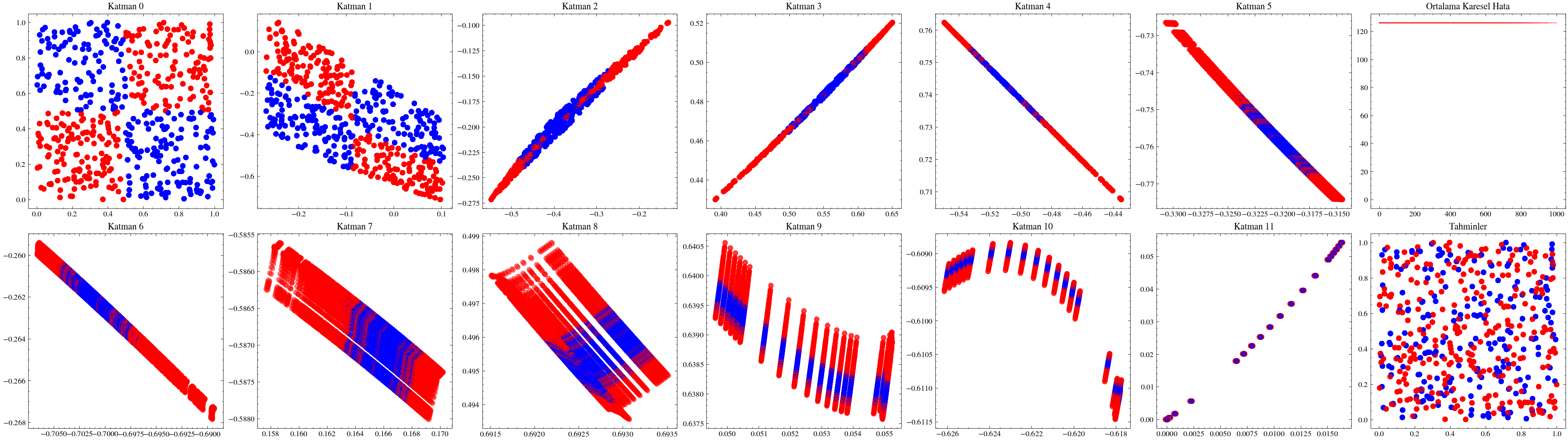
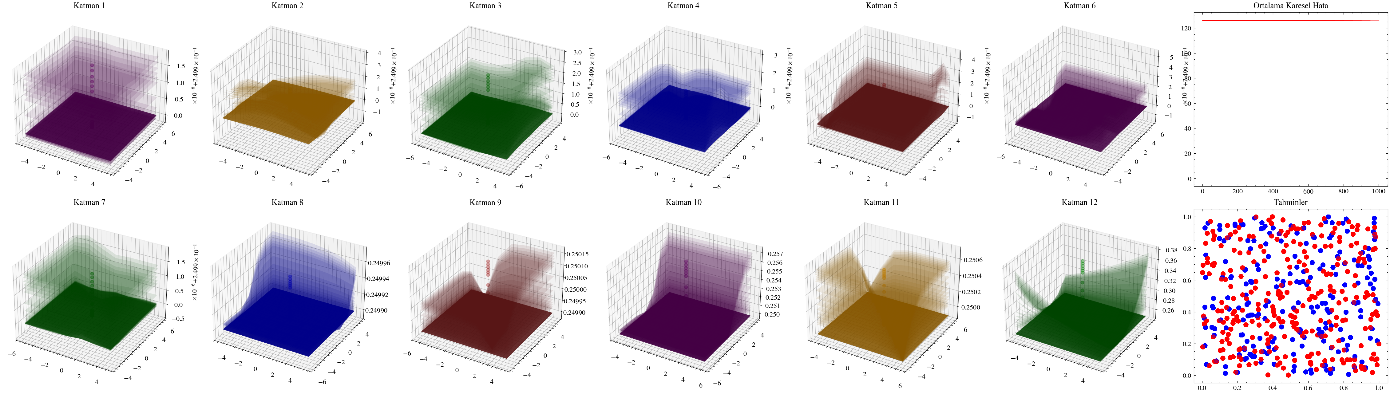
Aşağıdaki görselleştirmelerde, ilk katmanların kaybolan gradyanlar nedeniyle neredeyse hiç güncellenmediğini göreceğiz.

Image(filename=transformations_plot_filename)

Image(filename=loss_landscape_plot_filename)