Lojistik Regresyon

Lojistik regresyon, en uygun ağırlıklar ile sabit terimi (bias) öğrenerek iki sınıfa ait olasılıkları döndüren bir ikili sınıflandırma modelidir.

# import numpy as np
import autograd.numpy as np
from autograd import grad
from autograd import elementwise_grad as egrad

%matplotlib inline
import matplotlib.pyplot as plt
from mpl_toolkits.mplot3d import Axes3D

import sklearn.datasets as skdatasets

from celluloid import Camera
import scienceplots
from IPython.display import Image

np.random.seed(0)
plt.style.use(["science", "no-latex"])

Eğitim Veri Kümesi

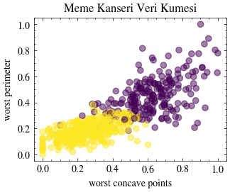
Meme kanseri veri kümesini içe aktaralım. Lojistik regresyon, tümörün ortalama çevresi ve ortalama yarıçapını kullanarak ikili sınıflandırma yapacak.

dataset = skdatasets.load_breast_cancer()

features_used = [-3, -8]
X = dataset.data[:, features_used]
feature_names = dataset.feature_names[features_used]

# min-max normalize the features along the columns
X_min_vals = X.min(axis=0)
X_max_vals = X.max(axis=0)
X = (X - X_min_vals) / (X_max_vals - X_min_vals)

Y = dataset.target
target_names = dataset.target_names

fig = plt.figure()
ax = fig.add_subplot()

ax.scatter(X[:, 0], X[:, 1], c=Y, alpha=0.5)
ax.set_xlabel(feature_names[0])
ax.set_ylabel(feature_names[1])
ax.set_title("Meme Kanseri Veri Kümesi")

Text(0.5, 1.0, 'Meme Kanseri Veri Kümesi')

Aktivasyon Fonksiyonu

Perceptron’un çıktısının, ağırlık vektörü \(\vec{w}\) ile giriş vektörü \(\vec{x}\) arasındaki skaler çarpıma sabit bir bias terimi \(b\) eklenmesiyle elde edildiğini hatırlayalım.

Perceptron: \(y=w^Tx + b\)

Aktivasyon fonksiyonları, bu hesaplamanın ardından uygulanır.

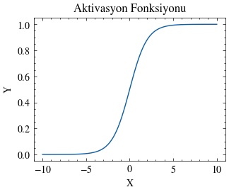
Sigmoid Fonksiyonu

İkili sınıflandırma yapabilmek için çıktı değerini (0, 1) aralığında tutmak ve hangi sınıfa ait olduğuna dair bir olasılık üretmek isteriz. Sigmoid fonksiyonu bunun için oldukça uygundur.

\( \sigma(z) = \frac{1}{1+e^-z} \)

sigmoid = lambda x: 1 / (1 + np.exp(-x))

def plot(fx, x_min, x_max, points=100, title=""):

    x = np.linspace(x_min, x_max, points)
    y = fx(x)

    fig, axes = plt.subplots()
    axes.plot(x, y)
    axes.set_xlabel("X")
    axes.set_ylabel("Y")
    axes.set_title("Aktivasyon Fonksiyonu")


x_min = -10
x_max = 10
points = 100
plot(sigmoid, x_min, x_max, points)

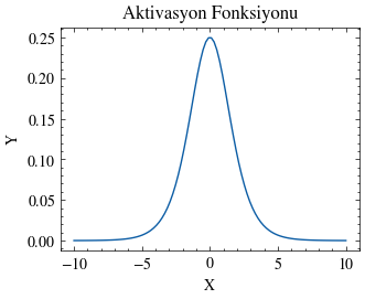
Sigmoid Fonksiyonunun Türevi

Birazdan en uygun ağırlıkları bulmak için gradyan inişini kullanacağız. Bu yüzden önce sigmoid fonksiyonunun türevini hesaplayalım.

\( \begin{align*} \sigma^\prime &= \frac{\partial}{\partial z} \sigma(z) \\ &= \frac{\partial}{\partial z} (\frac{1}{1+e^{-z}}) \\ &= \frac{\partial}{\partial z} (1+e^{-z})^{-1}) \\ &= (-1)(1+e^{-z})^{-2}\frac{\partial}{\partial z}(1+e^{-z}) \\ &= (-1)(1+e^{-z})^{-2}(e^{-z})\frac{\partial}{\partial z}(-z) \\ &= (-1)(1+e^{-z})^{-2}(e^{-z})(-1) \\ &= \frac{e^{-z}}{(1+e^{-z})^{2}} \end{align*} \)

sigmoid_prime = lambda x: np.exp(-x) / np.power((1 + np.exp(-x)), 2)
plot(sigmoid_prime, x_min, x_max, points)

Autograd

İsterseniz bir NumPy fonksiyonunun türevini almak için autograd da kullanabilirsiniz. PyTorch ve JAX de benzer otomatik türev alma mekanizmaları sunar.

# grad() differentiates scalar inputs
sigmoid_prime_grad = grad(sigmoid)
# egrad() differentiates vectorized inputs
sigmoid_prime_egrad = egrad(sigmoid)

x = np.linspace(x_min, x_max, points)
assert sigmoid_prime_grad(x[0]) == sigmoid_prime(x[0])
assert np.allclose(sigmoid_prime_egrad(x), sigmoid_prime(x))

plot(sigmoid_prime_egrad, x_min, x_max, points)

Kayıp Fonksiyonu

Lojistik regresyonda ikili çapraz entropi kaybı kullanılır. Bu kayıp fonksiyonu, maksimum olabilirlik tahmininden türetilir.

İkili sınıflandırma modelinde, ilk sınıfa ait olma olasılığı; ağırlık vektörü \(\vec{w}\) ile giriş vektörü \(\vec{x}\) arasındaki skaler çarpıma bias terimi \(b\) eklendikten sonra sigmoid uygulanarak elde edilir. Diğer sınıfa ait olma olasılığı ise bunun 1’den çıkarılmasıdır.

\( P(Y=1 \mid \vec{x}; \vec{w}, b) = \sigma{(\vec{w} \cdot \vec{x} + b)} \)

\( P(Y=0 \mid \vec{x}; \vec{w}, b) = 1 - P(Y=1 \mid \vec{x}; \vec{w}, b) \)

Maksimum Olabilirlik Tahmini

Maksimum olabilirlik tahmini, eğitim verisini gözleme olasılığını en büyük yapan ağırlık ve bias değerlerini bulur.

\(\vec{w}\) ve \(b\) cinsinden doğru ikili tahmin olasılığı aşağıdaki gibi yazılır. Bu ifade Bernoulli dağılımı olarak da düşünülebilir.

\( P(Y \mid \vec{x}; \vec{w}, b) = [\sigma{(\vec{w} \cdot \vec{x} + b)}]^{y} [1 - \sigma{(\vec{w} \cdot \vec{x} + b)}]^{1-y} \)

Eğitim verisinde \(n\) adet \(\vec{x_i}\) özelliği ve bunlara karşılık gelen \(y_i\) etiketleri varsa, toplam olasılık tüm örneklerin olasılıklarının çarpımı olarak yazılır. Bunu, mevcut ağırlık ve bias değerleri altında eğitim verisinin olabilirliği olarak düşünebilirsiniz.

\( P(Y \mid \vec{x_i}; \vec{w}, b) = \prod_{i=1}^{n} [\sigma{(\vec{w} \cdot \vec{x_i} + b)}]^{y_i} [1 - \sigma{(\vec{w} \cdot \vec{x_i} + b)}]^{1-y_i} \)

Amacımızın, toplam olabilirliği en büyük yapan en uygun \(\vec{w}\) ve \(b\) parametrelerini bulmak olduğunu unutmayın.

\( P(Y \mid \vec{x_i}; \vec{w}, b) = \max_{\vec{w}, b} \prod_{i=1}^{n} [\sigma{(\vec{w} \cdot \vec{x_i} + b)}]^{y_i} [1 - \sigma{(\vec{w} \cdot \vec{x_i} + b)}]^{1-y_i} \)

Lojistik regresyon modeli için en uygun ağırlık ve bias değerlerini bulmak amacıyla, optimizasyon problemlerini çözmekte kullanılan gradyan inişine başvururuz. Bunun için olabilirlik ifadesinin \(\vec{w}\) ve \(b\)’ye göre kısmi türevlerini almamız gerekir.

Ancak mevcut haliyle toplam olasılık çok sayıda çarpımdan oluşur. Çarpım kuralı nedeniyle türevler de oldukça karmaşık hale gelir. Bunu sadeleştirmek için olabilirliğin logaritmasını alırız; böylece çarpımlar toplamlara dönüşür.

\( \begin{align*} \ln(P(Y \mid \vec{x_i}; \vec{w}, b)) &= \max_{\vec{w}, b} \ln(\prod_{i=1}^{n} [\sigma{(\vec{w} \cdot \vec{x_i} + b)}]^{y_i} [1 - \sigma{(\vec{w} \cdot \vec{x_i} + b)}]^{1-y_i}) \\ &= \max_{\vec{w}, b} \sum_{i=1}^{n}[ \ln([\sigma{(\vec{w} \cdot \vec{x_i} + b)}]^{y_i} [1 - \sigma{(\vec{w} \cdot \vec{x_i} + b)}]^{1-y_i})] \\ &= \max_{\vec{w}, b} \sum_{i=1}^{n}[ \ln([\sigma{(\vec{w} \cdot \vec{x_i} + b)}]^{y_i}) + \ln([1 - \sigma{(\vec{w} \cdot \vec{x_i} + b)}]^{1-y_i})] \\ &= \max_{\vec{w}, b} \sum_{i=1}^{n}[ y_i \ln(\sigma{(\vec{w} \cdot \vec{x_i} + b)}) + (1-y_i) \ln(1 - \sigma{(\vec{w} \cdot \vec{x_i} + b)})] \\ \end{align*} \)

O halde, olabilirliğin negatif logaritmasını (yani yukarıdaki ifadeyi -1 ile çarparak) ikili çapraz entropi kaybı olarak tanımlarız. Ayrıca bunu örnek sayısına bölerek \(n\) örneğin ortalama kaybını elde ederiz.

\( \begin{align*} L(\vec{w}, b) = -\frac{1}{n} \sum_{i=1}^{n}[ y_i \ln(\sigma{(\vec{w} \cdot \vec{x_i} + b)}) + (1-y_i) \ln(1 - \sigma{(\vec{w} \cdot \vec{x_i} + b)})] \end{align*} \)

İkili Çapraz Entropi Kayıp Fonksiyonu

\(\hat y = \sigma{(\vec{w} \cdot \vec{x} + b)} = \frac{1}{1+e^-(\vec{w} \cdot \vec{x} + b)}\) olduğunu hatırlayalım.

Kayıp hesabını sadeleştirmek için ifadeyi \(\hat y\) cinsinden yeniden yazalım:

\( \begin{align*} L(\hat y) &= -\frac{1}{n} \sum_{i=1}^{n} [y_i \ln(\hat y_i) + (1-y_i) \ln(1 - \hat y_i)] \end{align*} \)

def bce(y_true, y_pred):
    return -np.sum(y_true * np.log(y_pred) + (1 - y_true) * np.log(1 - y_pred))

Kayıp Fonksiyonu: \(W\) ve \(B\) Cinsinden

Kayıp fonksiyonunun \(\vec{w}\) ve \(b\)’ye göre kısmi türevini almadan önce, hesabı kolaylaştırmak için ifadeyi biraz sadeleştirelim.

\(\hat y = \sigma{(\vec{w} \cdot \vec{x} + b)} = \frac{1}{1+e^-(\vec{w} \cdot \vec{x} + b)}\)

\( \begin{align*} L(\vec{w}, b) &= -\frac{1}{n} \sum_{i=1}^{n}[ y_i \ln(\sigma{(\vec{w} \cdot \vec{x_i} + b)}) + (1-y_i) \ln(1 - \sigma{(\vec{w} \cdot \vec{x_i} + b)})] \\ &= -\frac{1}{n} \sum_{i=1}^{n}[ y_i \ln(\sigma{(\vec{w} \cdot \vec{x_i} + b)}) - y_i \ln(1 - \sigma{(\vec{w} \cdot \vec{x_i} + b)}) + \ln(1 - \sigma{(\vec{w} \cdot \vec{x_i} + b)})] \\ &= -\frac{1}{n} \sum_{i=1}^{n}[ y_i \ln(\frac{\sigma{(\vec{w} \cdot \vec{x_i} + b)}}{1 - \sigma{(\vec{w} \cdot \vec{x_i} + b)}}) + \ln(1 - \sigma{(\vec{w} \cdot \vec{x_i} + b)})] \\ &= -\frac{1}{n} \sum_{i=1}^{n}[ y_i \ln(\frac{\frac{1}{1+e^{-(\vec{w} \cdot \vec{x} + b)}}}{1 - \frac{1}{1+e^{-(\vec{w} \cdot \vec{x} + b)}}}) + \ln(1 - \frac{1}{1+e^{-(\vec{w} \cdot \vec{x} + b)}})] \\ &= -\frac{1}{n} \sum_{i=1}^{n} [y_i \ln(e^{\vec{w} \cdot \vec{x_i} + b}) + \ln(\frac{1}{1+e^{\vec{w} \cdot \vec{x_i} + b}})] \\ &= -\frac{1}{n} \sum_{i=1}^{n} [y_i (\vec{w} \cdot \vec{x_i} + b) - \ln(1+e^{\vec{w} \cdot \vec{x_i} + b})] \\ \end{align*} \)

Kayıp Fonksiyonunun Gradyanı

Kayıp fonksiyonunun \(W\)’ye göre türevi:

\( \begin{align*} \nabla_{W} [L(\vec{w}, b)] &= \nabla_{W} [-\frac{1}{n} \sum_{i=1}^{n} [y_i (\vec{w} \cdot \vec{x_i} + b) - \ln(1+e^{\vec{w} \cdot \vec{x_i} + b})]] \\ &= -\frac{1}{n} \sum_{i=1}^{n} [y_i \nabla_{W} [\vec{w} \cdot \vec{x_i} + b] - \nabla_{W}[\ln(1+e^{\vec{w} \cdot \vec{x_i} + b})]] \\ &= -\frac{1}{n} \sum_{i=1}^{n} [y_i x_i - (\frac{1}{1+e^{\vec{w} \cdot \vec{x_i} + b}}) \nabla_{W}[1+e^{\vec{w} \cdot \vec{x_i} + b}]] \\ &= -\frac{1}{n} \sum_{i=1}^{n} [y_i x_i - (\frac{1}{1+e^{\vec{w} \cdot \vec{x_i} + b}}) (e^{\vec{w} \cdot \vec{x_i} + b})\nabla_{W}[\vec{w} \cdot \vec{x_i} + b]] \\ &= -\frac{1}{n} \sum_{i=1}^{n} [y_i x_i - (\frac{1}{1+e^{\vec{w} \cdot \vec{x_i} + b}}) (e^{\vec{w} \cdot \vec{x_i} + b})(x_i)] \\ &= -\frac{1}{n} \sum_{i=1}^{n} [y_i x_i - x_i(\frac{e^{\vec{w} \cdot \vec{x_i} + b}}{1+e^{\vec{w} \cdot \vec{x_i} + b}})] \\ &= -\frac{1}{n} \sum_{i=1}^{n} [y_i x_i - x_i(\frac{1}{1+e^{-(\vec{w} \cdot \vec{x_i} + b)}})] \\ &= -\frac{1}{n} \sum_{i=1}^{n} [y_i x_i - x_i\hat y_i] \\ &= \frac{1}{n} \sum_{i=1}^{n} [\hat y_i x_i - y_i x_i ] \\ &= \frac{1}{n} \sum_{i=1}^{n} [x_i (\hat y_i - y_i)] \\ \end{align*} \)

def bce_dw(x, y_true, y_pred):
    return np.mean(x * (y_pred - y_true))

Kayıp fonksiyonunun \(b\)’ye göre türevi:

\( \begin{align*} \frac{\partial}{\partial b} [L(\vec{w}, b)] &= \frac{\partial}{\partial b} [-\frac{1}{n} \sum_{i=1}^{n} [y_i (\vec{w} \cdot \vec{x_i} + b) - \ln(1+e^{\vec{w} \cdot \vec{x_i} + b})]] \\ &= -\frac{1}{n} \sum_{i=1}^{n} [y_i \frac{\partial}{\partial b} [\vec{w} \cdot \vec{x_i} + b] - \frac{\partial}{\partial b}[\ln(1+e^{\vec{w} \cdot \vec{x_i} + b})]] \\ &= -\frac{1}{n} \sum_{i=1}^{n} [y_i (1) - (\frac{1}{1+e^{\vec{w} \cdot \vec{x_i} + b}}) \frac{\partial}{\partial b}[1+e^{\vec{w} \cdot \vec{x_i} + b}] ] \\ &= -\frac{1}{n} \sum_{i=1}^{n} [y_i - (\frac{1}{1+e^{\vec{w} \cdot \vec{x_i} + b}}) (e^{\vec{w} \cdot \vec{x_i} + b}) \frac{\partial}{\partial b}[\vec{w} \cdot \vec{x_i} + b]] \\ &= -\frac{1}{n} \sum_{i=1}^{n} [y_i - (\frac{1}{1+e^{\vec{w} \cdot \vec{x_i} + b}}) (e^{\vec{w} \cdot \vec{x_i} + b}) (1)] \\ &= -\frac{1}{n} \sum_{i=1}^{n} [y_i - (\frac{e^{\vec{w} \cdot \vec{x_i} + b}}{1+e^{\vec{w} \cdot \vec{x_i} + b}})] \\ &= -\frac{1}{n} \sum_{i=1}^{n} [y_i - (\frac{1}{1+e^-({\vec{w} \cdot \vec{x_i} + b})})] \\ &= -\frac{1}{n} \sum_{i=1}^{n} [y_i - \hat y_i] \\ &= \frac{1}{n} \sum_{i=1}^{n} (\hat y_i - y_i) \\ \end{align*} \)

def bce_db(y_true, y_pred):
    return np.mean(y_pred - y_true)

Gradyan İnişi

İkili çapraz entropi kaybının \(\vec{w}\) ve \(b\) açısından türevlerini bulduğumuza göre, gradyan inişi denklemleri şöyle yazılır:

Ağırlıklar \(\vec{w}\) için gradyan inişi:

\( \begin{align*} \vec{w} &= \vec{w} - \eta \nabla_{W} [L(\vec{w}, b)] \\ &= \vec{w} - \eta [\frac{1}{n} \sum_{i=1}^{n} [x_i (\hat y_i - y_i)]] \end{align*} \)

Bias terimi \(b\) için gradyan inişi:

\( \begin{align*} b &= b - \eta \frac{\partial}{\partial b} [L(\vec{w}, b)] \\ &= b - \eta [\frac{1}{n} \sum_{i=1}^{n} (\hat y_i - y_i)] \end{align*} \)

def gradient_descent(weights, x, bias, y_true, y_pred, learning_rate):
    weights = weights - learning_rate * bce_dw(x, y_true, y_pred)
    bias = bias - learning_rate * bce_db(y_true, y_pred)

    return weights, bias

Grafik Fonksiyonları

Görselleştirmeleri üretmek için yardımcı fonksiyonlar.

def create_plots():
    fig, ax = plt.subplots(1, 3, figsize=(16 / 9.0 * 4, 4 * 1))
    fig.suptitle("Lojistik Regresyon")

    ax[0].set_xlabel("Epok", fontweight="normal")
    ax[0].set_ylabel("Hata", fontweight="normal")
    ax[0].set_title("İkili Çapraz Entropi Hatası")

    ax[1].axis("off")
    ax[2].axis("off")

    ax[2] = fig.add_subplot(1, 2, 2, projection="3d")
    ax[2].set_xlabel("X")
    ax[2].set_ylabel("Y")
    ax[2].set_zlabel("Z")
    ax[2].set_title("Tahmin Olasılıkları")
    ax[2].view_init(20, -35)

    camera = Camera(fig)
    return ax[0], ax[2], camera


def plot_graphs(
    ax0,
    ax1,
    idx,
    visible_mse,
    mse_idx,
    errors,
    features,
    labels,
    predictions,
    points_x,
    points_y,
    surface_predictions,
):
    ax0.plot(
        mse_idx[visible_mse][: idx + 1],
        errors[visible_mse][: idx + 1],
        color="red",
        alpha=0.5,
    )

    # Plot Logistic Regression Tahminler
    # Ground truth and training data
    ground_truth_legend = ax1.scatter(
        features[:, 0],
        features[:, 1],
        labels,
        color="red",
        alpha=0.5,
        label="Gerçek Etiket",
    )
    # Logistic Regression Tahminler
    predictions_legend = ax1.scatter(
        features[:, 0],
        features[:, 1],
        predictions,
        color="blue",
        alpha=0.2,
        label="Tahmin",
    )
    ax1.plot_surface(
        points_x,
        points_y,
        surface_predictions.reshape(dims, dims),
        color="blue",
        alpha=0.2,
    )
    ax1.legend(
        (ground_truth_legend, predictions_legend),
        ("Gerçek Etiket", "Tahminler"),
        loc="upper left",
    )

Modeli Eğitmek

def fit(
    w0, b0, features, labels, dims, epochs, learning_rate, optimizer, output_filename
):
    mse_idx = np.arange(1, epochs + 1)
    errors = np.full(epochs, -1)
    ax0, ax1, camera = create_plots()

    points = np.linspace(0, 1, dims)
    points_x, points_y = np.meshgrid(points, points)
    surface_points = np.column_stack((points_x.flatten(), points_y.flatten()))

    weights = w0
    bias = b0

    for idx in range(epochs):
        error = 0
        predictions = np.array([])
        surface_predictions = np.array([])

        # fit the model on the training data
        for x, y in zip(features, labels):
            output = sigmoid(np.dot(weights, x) + bias)

            predictions = np.append(predictions, output)

            # Store Hata
            error += bce(y, output)

            # Gradyan İnişi
            weights, bias = optimizer(weights, x, bias, y, output, learning_rate)

        # error /= len(features)

        # Visualization
        if (
            idx < 5
            or (idx < 15 and idx % 5 == 0)
            or (idx <= 50 and idx % 25 == 0)
            or (idx <= 1000 and idx % 200 == 0)
            or idx % 500 == 0
        ):
            for surface_point in surface_points:
                output = sigmoid(np.dot(weights, surface_point) + bias)
                surface_predictions = np.append(surface_predictions, output)

            print(f"epok: {idx:>4}, BCE: {round(error, 2)}")

            # Plot BCE
            errors[idx] = error
            visible_mse = errors != -1

            plot_graphs(
                ax0,
                ax1,
                idx,
                visible_mse,
                mse_idx,
                errors,
                features,
                labels,
                predictions,
                points_x,
                points_y,
                surface_predictions,
            )

            camera.snap()

    animation = camera.animate()
    animation.save(output_filename, writer="pillow")

epochs = 5001
learning_rate = 0.0005
dims = 10

w0 = np.random.rand(X[0].shape[0])
b0 = np.random.rand()

output_filename = "logistic_regression.gif"
fit(w0, b0, X, Y, dims, epochs, learning_rate, gradient_descent, output_filename)

epok:    0, BCE: 444.23
epok:    1, BCE: 438.52
epok:    2, BCE: 433.32
epok:    3, BCE: 428.58
epok:    4, BCE: 424.25
epok:    5, BCE: 420.28
epok:   10, BCE: 404.5
epok:   25, BCE: 375.53

epok:   50, BCE: 341.83

epok:  200, BCE: 231.95

epok:  400, BCE: 176.56

epok:  500, BCE: 161.66

epok:  600, BCE: 150.72

epok:  800, BCE: 135.71

epok: 1000, BCE: 125.86

epok: 1500, BCE: 111.57

epok: 2000, BCE: 103.85

epok: 2500, BCE: 99.03

epok: 3000, BCE: 95.75

epok: 3500, BCE: 93.39

epok: 4000, BCE: 91.61

epok: 4500, BCE: 90.24

epok: 5000, BCE: 89.16

Image(filename=output_filename)